Real Datasets

Introduction

This section details real-world datasets which are illustrative of the power behind DHARMa residuals. It is recommended that you read the “Getting Started” page before continuing here.

To run the code in this section, you will first have to install some packages. You can skip this step if you already have these.

#### Specify Packages to Load ####
pkgs <- c(
  "SuppDists", "DHARMa", "ggfortify",
  "MASS", "tidyverse", "mgcv", "see",
  "lmerTest", "ggrain", "MPsychoR",
  "gamlss", "gamlss.data"
  )

#### Install Packages ####
install.packages(pkgs)

Then you just need to load the packages so you can use the functions from them.

#### Libraries ####
library(mgcv) # for GAMs
library(DHARMa) # for DHARMa residuals
library(MASS) # for NB models
library(tidyverse) # for wrangling
library(ggfortify) # for ggplot2-style plots of standard residual checks
library(performance) # for checking model performance
library(lmerTest) # for mixed modeling functions
library(MPsychoR) # for IAT data
library(ggrain) # for raincloud plots
library(gamlss) # for GAMLSS models
library(gamlss.data) # for GAMLSS data

#### Get Datasets ####
data("iatfaces")
data("rent")

#### Set Plot Theme ####
set_theme(theme_classic(base_size = 16)) # for stylizing plots

Dataset 1: GLM with Non-Normal Count Response

Explanation of Data Context

This data was obtained from an original dataset in Linguistic Diversity and the R book Statistics for Linguists, which has a variety of datasets related to linguistics and psycholinguistics (Nettle, 1999; Winter, 2019). To simplify things, I provide the code to reconstruct the data so that it is immediately usable in your R session in tidy format.

#### Create Tibble of Nettle Data ####
nettle <- tibble(
  Country = c(
    "Algeria", "Angola", "Australia", "Bangladesh", "Benin", "Bolivia",
    "Botswana", "Brazil", "Burkina Faso", "CAR", "Cambodia", "Cameroon", "Chad",
    "Colombia", "Congo", "Costa Rica", "Cote d'Ivoire", "Cuba", "Ecuador",
    "Egypt", "Ethiopia", "French Guiana", "Gabon", "Ghana", "Guatemala", "Guinea",
    "Guyana", "Honduras", "India", "Indonesia", "Kenya", "Laos", "Liberia",
    "Libya", "Madagascar", "Malawi", "Malaysia", "Mali", "Mauritania", "Mexico",
    "Mozambique", "Myanmar", "Namibia", "Nepal", "Nicaragua", "Niger", "Nigeria",
    "Oman", "Panama", "Papua New Guinea", "Paraguay", "Peru", "Philippines",
    "Saudi Arabia", "Senegal", "Sierra Leone", "Solomon Islands", "Somalia",
    "South Africa", "Sri Lanka", "Sudan", "Suriname", "Tanzania", "Thailand",
    "Togo", "UAE", "Uganda", "Vanuatu", "Venezuela", "Vietnam", "Yemen", "Zaire",
    "Zambia", "Zimbabwe"
  ),
  Population = c(
    4.41, 4.01, 4.24, 5.07, 3.69, 3.88, 3.13, 5.19, 3.97, 3.5, 3.93, 4.09, 3.76,
    4.53, 3.37, 3.49, 4.1, 4.03, 4.04, 4.74, 4.73, 2.01, 3.08, 4.19, 3.98, 3.77,
    2.9, 3.72, 5.93, 5.27, 4.41, 3.63, 3.43, 3.67, 4.06, 3.93, 4.26, 3.98, 3.31,
    4.94, 4.21, 4.63, 3.26, 4.29, 3.6, 3.9, 5.05, 3.19, 3.39, 3.58, 3.64, 4.34,
    4.8, 4.17, 3.88, 3.63, 3.52, 3.89, 4.56, 4.24, 4.41, 2.63, 4.45, 4.75, 3.56,
    3.21, 4.29, 2.21, 4.31, 4.83, 4.09, 4.56, 3.94, 4
  ),
  Area = c(
    6.38, 6.1, 6.89, 5.16, 5.05, 6.04, 5.76, 6.93, 5.44, 5.79, 5.26, 5.68, 6.11,
    6.06, 5.53, 4.71, 5.51, 5.04, 5.45, 6, 6.09, 4.95, 5.43, 5.38, 5.04, 5.39,
    5.33, 5.05, 6.52, 6.28, 5.76, 5.37, 5.05, 6.25, 5.77, 5.07, 5.52, 6.09, 6.01,
    6.29, 5.9, 5.83, 5.92, 5.15, 5.11, 6.1, 5.97, 5.33, 4.88, 5.67, 5.61, 6.11,
    5.48, 6.33, 5.29, 4.86, 4.46, 5.8, 6.09, 4.82, 6.4, 5.21, 5.98, 5.71, 4.75,
    4.92, 5.37, 4.09, 5.96, 5.52, 5.72, 6.37, 5.88, 5.59
  ),
  MGS = c(
    6.6, 6.22, 6, 7.4, 7.14, 6.92, 4.6, 9.71, 5.17, 8.08, 8.44, 9.17, 4, 11.37,
    9.6, 8.92, 8.67, 7.46, 8.14, 0.89, 7.28, 10.4, 8.79, 8.79, 9.31, 7.38, 12,
    8.54, 5.32, 10.67, 7.26, 7.14, 10.62, 2.43, 7.33, 5.8, 11.92, 3.59, 0.75,
    5.84, 6.07, 6.93, 2.5, 6.39, 8.13, 2.4, 7, 0, 9.2, 10.88, 10.25, 2.65, 10.34,
    0.4, 3.58, 8.22, 12, 3, 6.05, 9.59, 4.02, 12, 7.02, 8.04, 7.91, 0.83, 10.14,
    12, 7.98, 8.8, 0, 9.44, 5.43, 5.29
  ),
  Langs = c(
    18L, 42L, 234L, 37L, 52L, 38L, 27L, 209L, 75L, 94L, 18L, 275L, 126L, 79L, 60L,
    10L, 75L, 1L, 22L, 11L, 112L, 11L, 40L, 73L, 52L, 29L, 14L, 9L, 405L, 701L,
    58L, 93L, 34L, 13L, 4L, 14L, 140L, 31L, 8L, 243L, 36L, 105L, 21L, 102L, 7L,
    21L, 427L, 8L, 13L, 862L, 21L, 91L, 168L, 8L, 42L, 23L, 66L, 14L, 32L, 7L,
    134L, 17L, 131L, 82L, 43L, 9L, 43L, 111L, 40L, 88L, 6L, 219L, 38L, 18L
  ),
)

#### Print Data ####
nettle

# A tibble: 74 × 5
   Country      Population  Area   MGS Langs
   <chr>             <dbl> <dbl> <dbl> <int>
 1 Algeria            4.41  6.38  6.6     18
 2 Angola             4.01  6.1   6.22    42
 3 Australia          4.24  6.89  6      234
 4 Bangladesh         5.07  5.16  7.4     37
 5 Benin              3.69  5.05  7.14    52
 6 Bolivia            3.88  6.04  6.92    38
 7 Botswana           3.13  5.76  4.6     27
 8 Brazil             5.19  6.93  9.71   209
 9 Burkina Faso       3.97  5.44  5.17    75
10 CAR                3.5   5.79  8.08    94
# ℹ 64 more rows

As one can see, the data contains 5 variables:

Country: The country which the data comes from.
Population: The number of people in a country.
Area: The size of the country.
MGS: Mean growing season.
Langs: The number of languages in a country.

We will use this data to test the Nettle Hypothesis, which is that a country’s agricultural reliability (e.g. how available crops are in a given year) predicts a country’s linguistic diversity. To do this, we will try to predict the number of languages in a country based on the mean growing season (MGS) of that country. The assumption under the Nettle Hypothesis is that the longer the MGS, the more languages are used in a country.

We can quickly visualize these variables to see what the distribution looks like with some simple code…

plot(
  nettle$MGS,
  nettle$Langs,
  main = "Languages by MGS",
  xlab = "Mean Growing Season (MGS)",
  ylab = "Languages",
  col = "gray",
  pch = 19
)

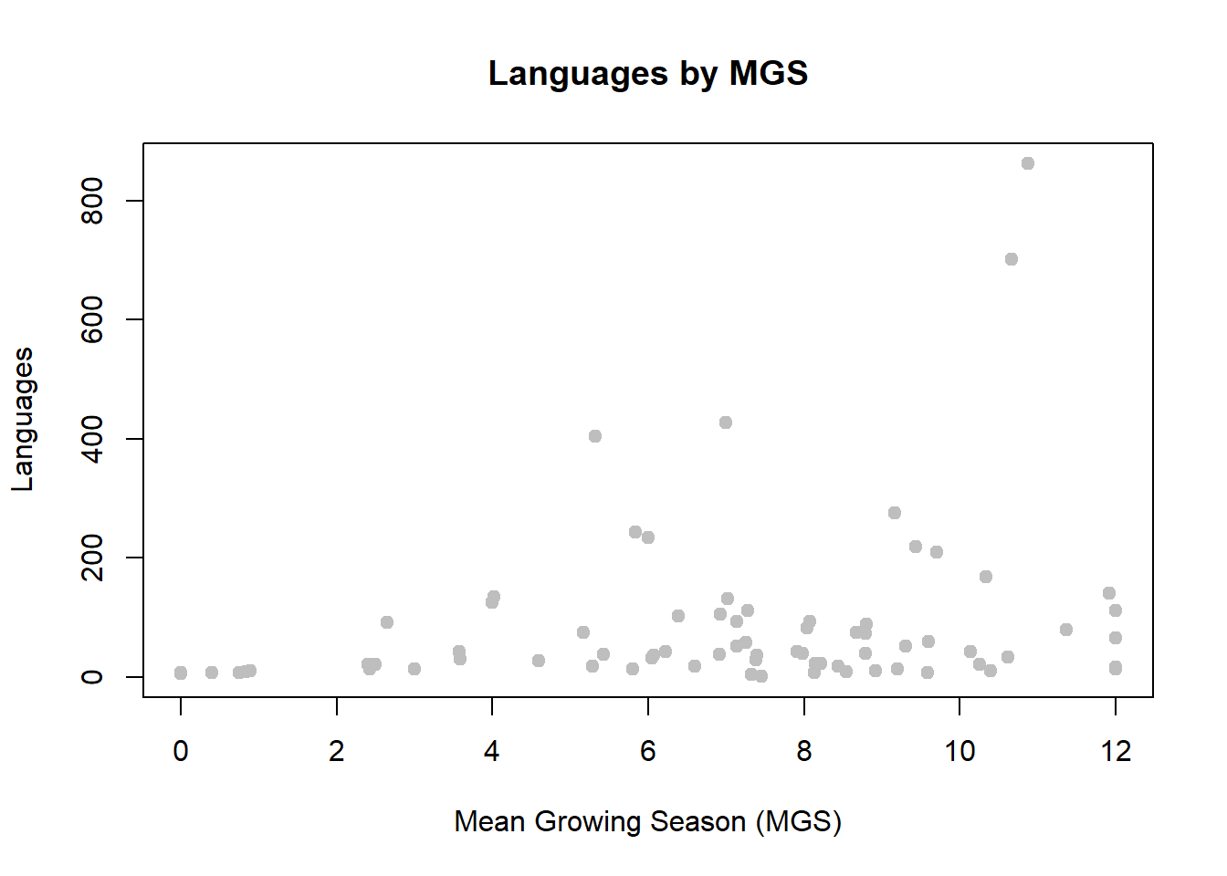
We can see that the association isn’t totally clear, but given the data piles up at the bottom, the response is very likely to be right-skewed. We can easily check this ourselves with a histogram.

hist(
  nettle$Langs,
  xlab = "Languages",
  main = "Distribution of Languages"
)

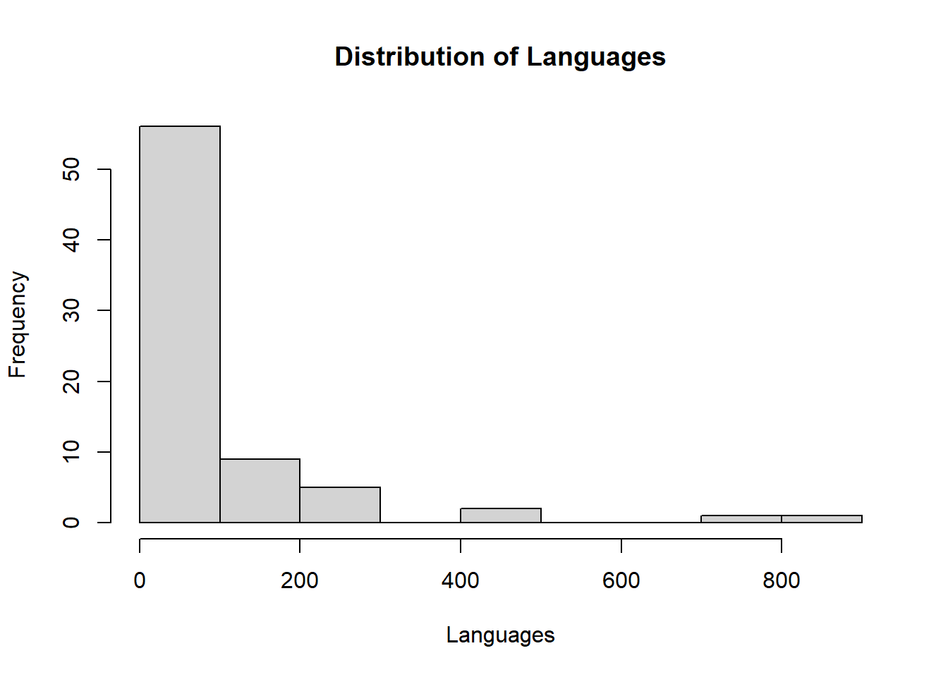
As we see here, the distribution is clearly right skewed, and given languages are a discrete count, it probably makes sense to start off with models which predict this kind of data.

Model 1: Using a Naive OLS Model

We will first begin with a “standard” ordinary least squares (OLS) regression model by using the lm() function.

#### Fit Poor Model ####
fit.poor <- lm(
  formula = Langs ~ MGS,
  data = nettle
)

Then we will use our DHARMa residuals to check the model fitness.

sim.poor <- simulateResiduals(fit.poor)
plot(sim.poor)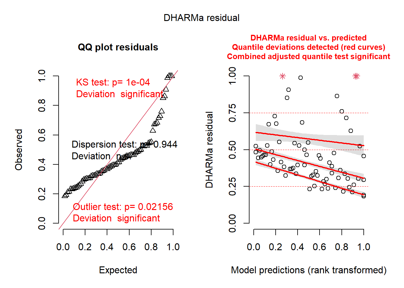

It is clear this model is mistfit because the points on the left plot deviate a lot from the QQ line and the right plot has some odd patterns. Since the quantile regression lines are not horizontal and parallel to each other, we can try to improve upon this model with some adjustments.

Model 2: Fitting a Count Process with a Standard Poisson Model

A Poisson generalized linear model (GLM) is often advised as a first step for modeling counts (Gelman et al., 2022), which we will use here now. All this takes is switching to the glm() function and adding in family = 'poisson' or family = poisson() to the function.

#### Fit Basic Poisson ####
fit.poiss.1 <- glm(
  formula = Langs ~ MGS,
  data = nettle,
  family = 'poisson'
  )

Once again, we will assess the model fit with DHARMa.

sim.poiss.1 <- simulateResiduals(fit.poiss.1)
plot(sim.poiss.1)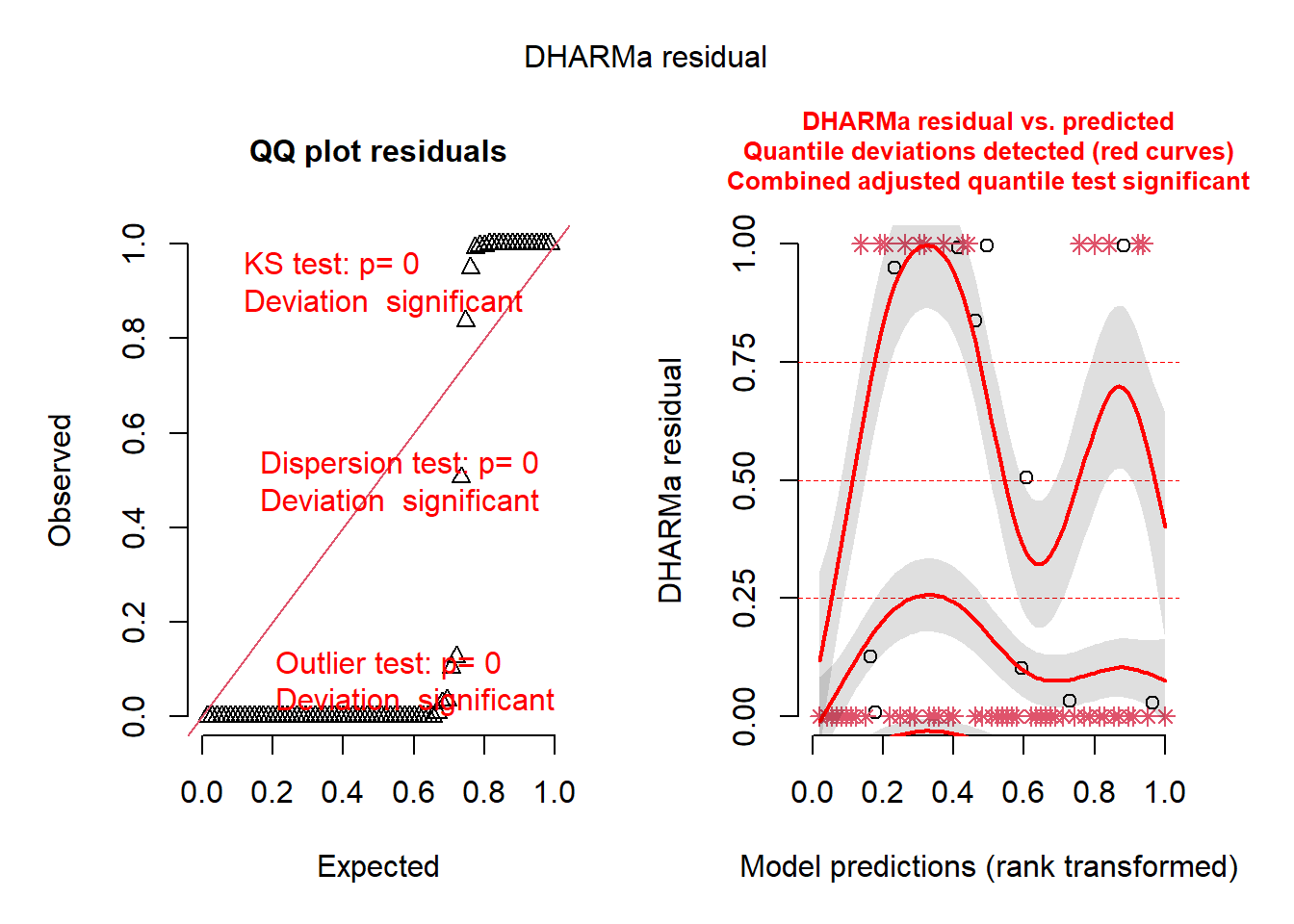

The residuals look even worse in this model. It is common in Poisson models that the variance exceeds the mean (overdispersion). We should check that this is not the case before moving on. We can use the testDispersion() function to figure this out (see Get Started page for more info).

testDispersion(fit.poiss.1)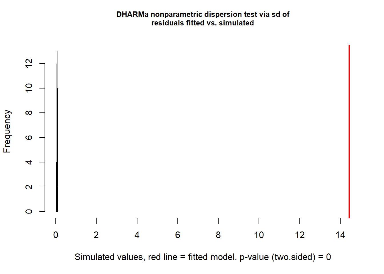


    DHARMa nonparametric dispersion test via sd of residuals fitted vs.
    simulated

data:  simulationOutput
dispersion = 219.78, p-value < 2.2e-16
alternative hypothesis: two.sided

The output tells us that the dispersion is insane…it is 219.78. For perspective, we want this number to be as close to 1 as possible. Correspondingly, our histogram shows a red line which is far to the right. We normally want this to be as close to the center of the histogram as possible. Therefore, we will have to look closer at the data to see why this count model performs so much worse than our OLS model.

Model 3: Adding an Offset to the Model

If we look closer, the data includes a variable called Area to measure the size of a country. It could be that the data generating process (DGP) is best captured as a ratio (languages per square mile) rather than a count of languages alone. This is because countries with a larger land mass tend to have more languages spoken in them (Winter, 2019). Therefore, it may be beneficial to control for this in some way by adding it into the model.

Ratios can be modeled by adding the offset() function and plugging in the variable that adjusts our count. In this case, we just add offset(Area) to our previous formula.

#### Fit Exposure Model ####
fit.poiss.2 <- glm(
  Langs ~ MGS + offset(Area),
  data = nettle,
  family= 'poisson'
  )

We once again turn to DHARMa to see if the model has improved.

sim.poiss.2 <- simulateResiduals(fit.poiss.2)
plot(sim.poiss.2)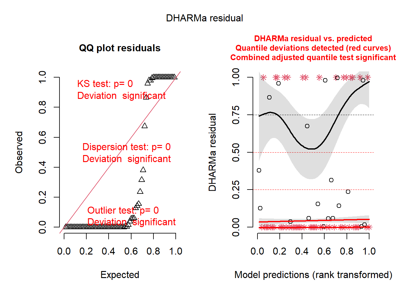

While this model is probably marginally better, it still is nowhere close to ideal. Let’s see if dispersion is still an issue.

testDispersion(fit.poiss.2)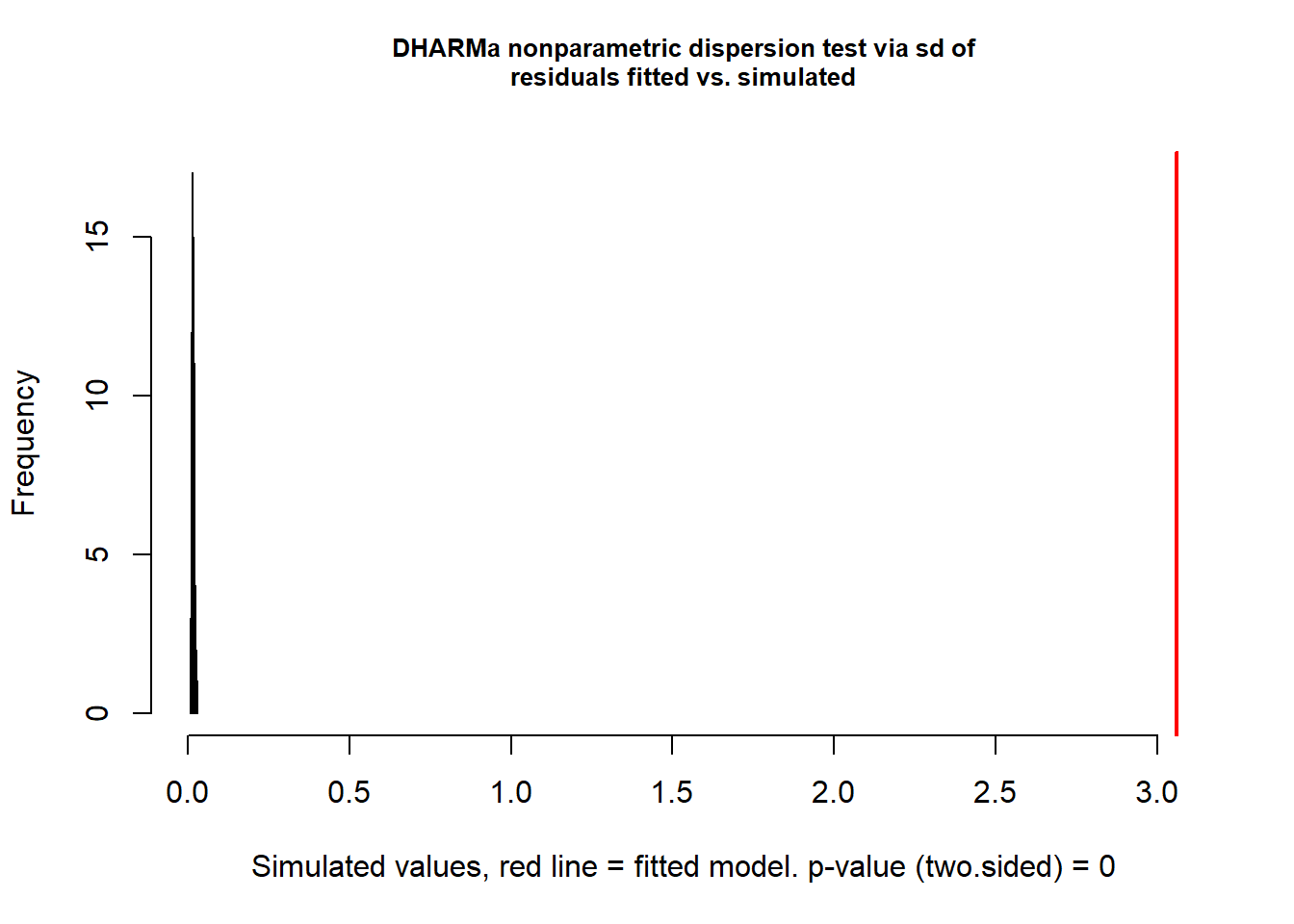


    DHARMa nonparametric dispersion test via sd of residuals fitted vs.
    simulated

data:  simulationOutput
dispersion = 173.54, p-value < 2.2e-16
alternative hypothesis: two.sided

The good news is that our dispersion has decreased dramatically. The bad news is that it is still extremely high (173.54). Therefore, we need to find a more flexible model since our offset clearly didn’t fix our problem.

Model 4: Dealing with Overdispersion with an NB Model

One of the unfortunate realities of Poisson GLMs is that they are often overdispersed. These are consequently better modeled with a negative binomial GLM instead (Gelman et al., 2022), which we fit below. We switch to the MASS package’s glm.nb() function to use this kind of model.

#### Fit Exposure Model ####
fit.nb <- glm.nb(
  Langs ~ MGS + offset(Area),
  data = nettle
)

Once again, we check the model with DHARMa.

sim.nb <- simulateResiduals(fit.nb)
plot(sim.nb)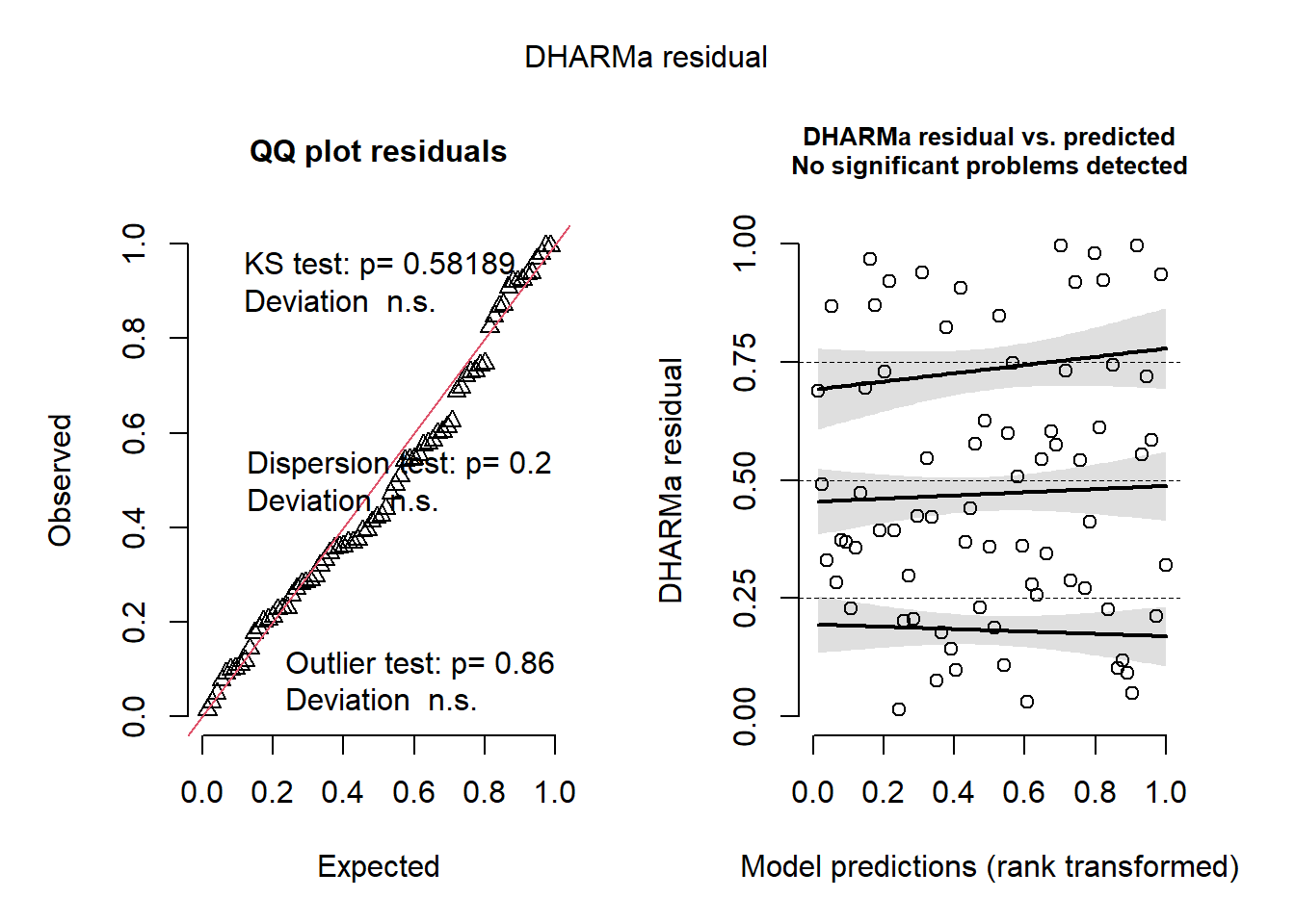

Our model looks to have substantial improvement compared to before. Let’s look at the dispersion parameter once more to see if this is now diminished.

testDispersion(fit.nb)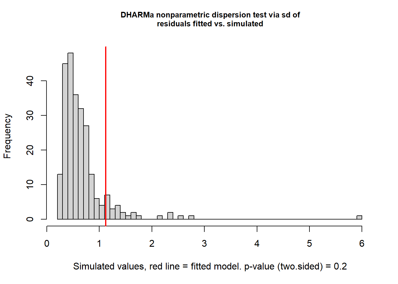


    DHARMa nonparametric dispersion test via sd of residuals fitted vs.
    simulated

data:  simulationOutput
dispersion = 1.6765, p-value = 0.2
alternative hypothesis: two.sided

Here we find the most dramatic change in dispersion. It is now about 1.68. While this could still be cause for concern, this model is already a gigantic improvement over the past iterations and is probably already safe. To explore how we can get the dispersion down to a lower value, see the “Bonus: Fitting a PIG Model for Extreme Skew” under the “Custom DHARMa Residuals for GAMLSS” section.

Final Comparison of Models and Plot

We can compare all of the model fits with the following code. The invisible() function is used here to kill the messages generated by the code.

par(mfrow=c(2,4))
invisible(testUniformity(fit.poor))
invisible(testUniformity(fit.poiss.1))
invisible(testUniformity(fit.poiss.2))
invisible(testUniformity(fit.nb))

invisible(testQuantiles(fit.poor))
invisible(testQuantiles(fit.poiss.1))
invisible(testQuantiles(fit.poiss.2))
invisible(testQuantiles(fit.nb))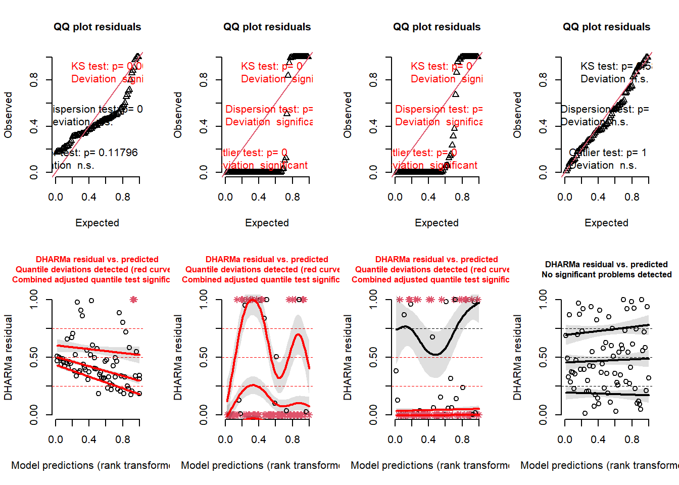

par(mfrow=c(1,1))

The plots suggest that our final fit with the negative binomial model performs best. This is followed by the original OLS model, which while not perfect, seems to outshine the Poisson models. The worst performer by far is the standard Poisson model without an offset. We can visualize the final negative binomial model with some ggplot2 code as well. The GAM argument and nb2() function from mgcv are used here for convenience, but it still plots what is essentially a GLM.

#### Create Plot ####
final.plot <- nettle %>% 
  ggplot(
    aes(
      x = MGS,
      y = Langs
    )
  )+
  geom_point(
    color = "gray",
    size = 5
    )+
  stat_smooth(
    color = "black",
    method = "gam",
    method.args = list(family = mgcv::nb()),
    formula = y ~ x
  )+
  labs(
    x = "Mean Growing Season (MGS)",
    y = "Languages",
    title = "Final NB GLM"
  )+
  scale_x_continuous(n.breaks = 12)

#### Print Plot ####
final.plot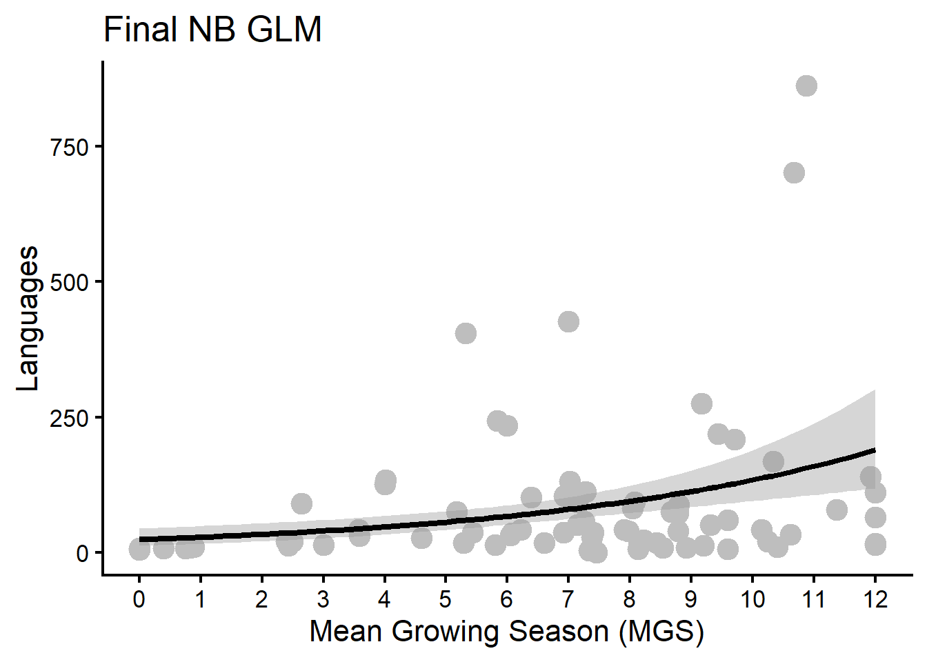

The plot shows that there is a positive trend. As the mean growing season in a country increases, the number of languages there increases. Plugging in some predictions for a couple of MGS values will make this clear.

predict(
  object =  fit.nb, # the fitted model
  newdata = data.frame(
    MGS = c(6, 12),
    Area = mean(nettle$Area)
    ), # the values we plug into the model
  type = "response" # convert to counts
)

        1         2 
 51.55121 204.42282

When the mean growing season is 6 months, the model predicts around 51 languages. When the mean growing season is year long (12 months), it predicts around 204 languages. This is a substantial increase.

Dataset 2: GLMM with Non-Normal Continuous Response

Explanation of the Data Context

This dataset was obtained from the R package MPsychoR and is one study from a series of studies on implicit association tests, or IATs (Greenwald & Banaji, 1995; Greenwald et al., 1998; Nosek et al., 2002). We can quickly glimpse the data to see what is inside.

glimpse(iatfaces)

Rows: 320
Columns: 4
$ block   <fct> congruent, congruent, congruent, congruent, congruent, congrue…
$ latency <dbl> 554, 703, 664, 503, 527, 577, 673, 607, 896, 575, 473, 623, 71…
$ id      <fct> 1, 1, 1, 1, 1, 1, 1, 1, 1, 1, 1, 1, 1, 1, 1, 1, 1, 1, 1, 1, 1,…
$ trial   <int> 1, 2, 3, 4, 5, 6, 7, 8, 9, 10, 11, 12, 13, 14, 15, 16, 17, 18,…

We can see it has 4 variables, and the help page for this data lists the following information for context:

The implicit association test (IAT) measures differential association of two target concepts with an attribute. In this experiment the participants saw images of people with long faces, images of people with wide faces, positively valenced words, and negatively valenced words. In the first critical block (“congruent block”), participants were asked to press one response key if they saw a long-faced person or a positive word and a different response key if they saw a wide-faced person or a negative word. In the second critical block (“incongruent block”), the pairing was reversed. Participants were asked to press one key for long-faced people or negative words and a different key for wide-faced people or positive words. IAT theory states that participants are expected to be able to respond fast in congruent conditions and slowly in incongruent conditions. The dataset contains trajectories of 4 participants. Each participant was exposed 80 trials: first, 40 congruent block trials, followed by 40 incongruent block trials. The response variable is latency.

Given this context, we can ask ourselves the question “Do incongruent pairs of stimuli increase latency (reaction times)?” According to IAT Theory, it seems plausible that incongruent pairs, what we are not expecting, would cause slower responses.

Model 1: Problems with Singularity

As multiple participants are exposed to each trial and each trial is exposed to multiple participants, this at first glance looks like a classic crossed random effects design (Baayen et al., 2008). We would normally begin by first fitting a standard linear mixed model with a Gaussian (normal) distribution using the lmer() function. The (1|RE) notation specifies that the model includes random intercepts for the given terms, here trial and subjects.

However, block and trial are not independent of each other and fitting both in the model will produce singularity issues, as seen below:

fit.singularity <- lmer(
  latency ~ block + (1|id) + (1|trial),
  data = iatfaces
)

boundary (singular) fit: see help('isSingular')

Therefore, the model will be simplified by only adding in subject ID as a random effect since the block is the theoretical predictor we would care about most in this model.

Model 2: Mis-Specified Distribution

We begin by sticking to the Gaussian distribution from lmer() as a default after dropping trials:

fit.iat.1 <- lmer(
  latency ~ block + (1|id),
  data = iatfaces
)

To check the model fit, we can explore the DHARMa residuals once more.

sim.iat.1 <- simulateResiduals(fit.iat.1)
plot(sim.iat.1)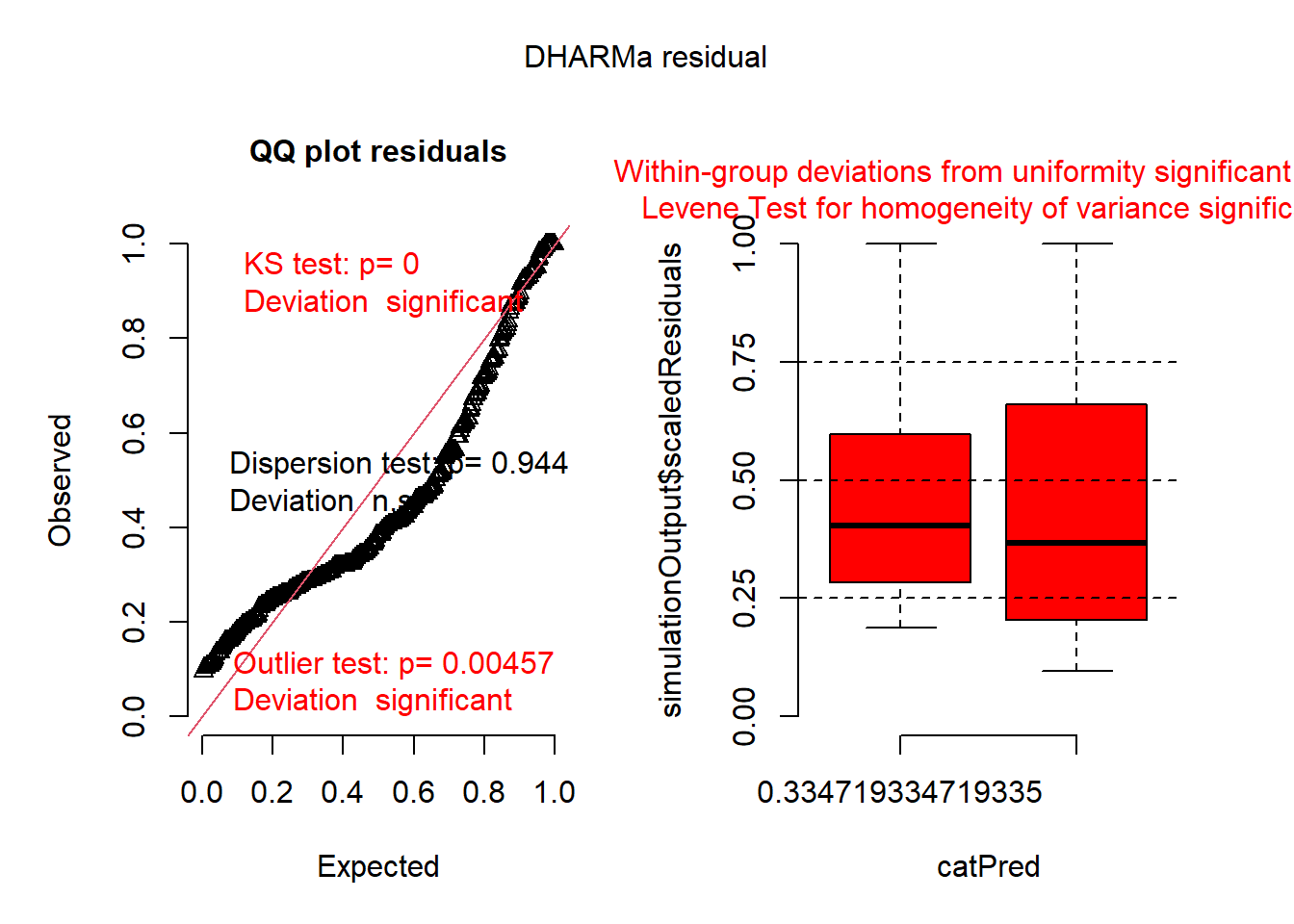

We see an issue with specification here already. The QQ line is clearly not matching the data points and the categorical predictor effects (congruent vs incongruent) seem to be off. This is because in the right plot, the medians of the boxplots should center around .50 generally and the limits of the boxplot should hover within the .25 and .75 quartiles. Observing the raw data, we can see a familiar pattern with latency data.

iatfaces %>% 
  ggplot(
    aes(
      x = block,
      y = latency
    )
  )+
  geom_rain()+
  coord_flip()+
  labs(
    y = "Latency",
    x = "Block",
    title = "Response Latency by Block"
  )+
  scale_y_continuous()+
  facet_wrap(~id)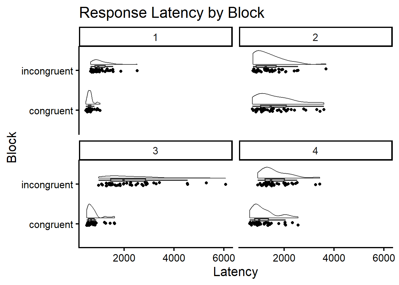

We see that across all 4 participants, the latencies have a continuous right-skewed distribution. This is normal, as they often take on a variety of distributions which are often (but not always) right-skewed (Baayen & Milin, 2010). These include the Gaussian, Gamma, inverse Gaussian, log-normal, and other well-documented distributions (see this website for practical examples). Which then do we choose?

Model 3: Attempting a Gamma Distribution

We can try to fit a Gamma distribution first to see if it will fix our model’s residuals. We use a log link here because the model once again fails to converge if you use the default inverse link function with family = Gamma(link = "inverse").

fit.iat.2 <- glmer(
  latency ~ block + (1|id),
  data = iatfaces,
  family = Gamma(link = "log")
)

Then we check the residuals once again.

sim.iat.2 <- simulateResiduals(fit.iat.2)
plot(sim.iat.2)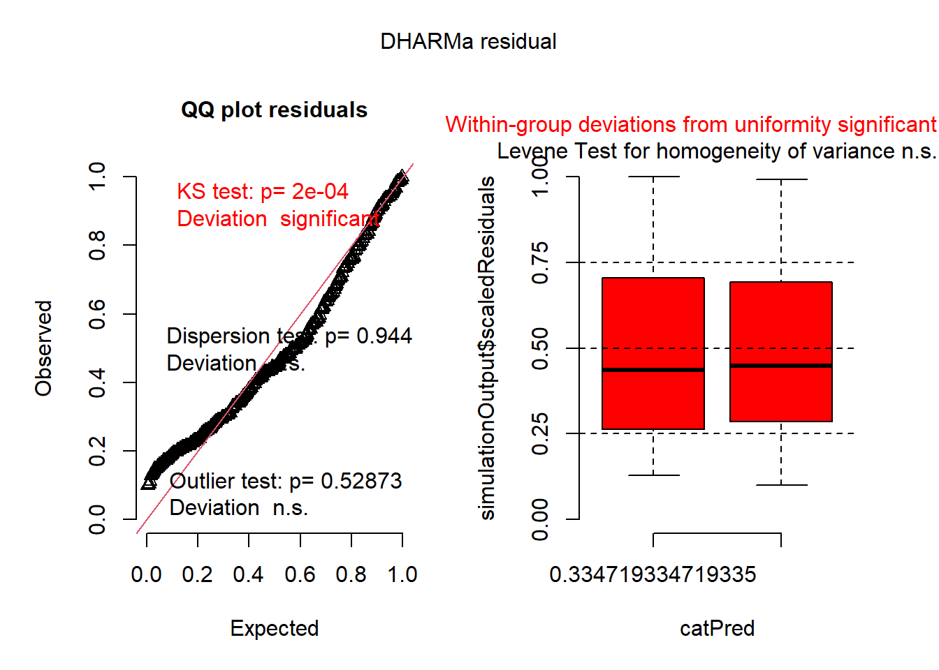

The model appears better but still isn’t perfect. Fitting to other skewed distributions results in similar or worse fits.

Model 4: Using an Interpretable and Better-Fitting Transformation

It is usually best to not blindly transform variables so they become normal. However, if we have a strong rationale guided by both theory and interpretation, then this is more acceptable. With latency / reaction time data, often an inverse RT is used instead (Baayen & Milin, 2010; Brysbaert & Stevens, 2018). This is calculated with the following formula:

\[ \text{Inverse RT} = \frac{-1000}{\text{RT}} \] The inverse RT now represents units of information processed per millisecond, which has the added benefit of normalizing the distribution in many cases. We can see this in action in the following model.

fit.iat.3 <- lmer(
  I(-1000/latency) ~ block + (1|id),
  data = iatfaces
)

And the residuals can once again be checked below:

sim.iat.3 <- simulateResiduals(fit.iat.3)
plot(sim.iat.3)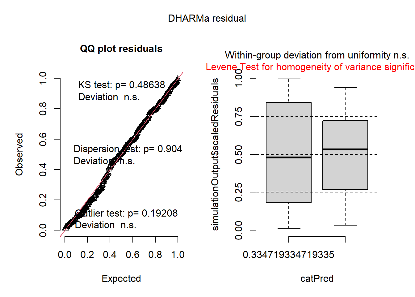

The model now fits considerably better. Though the Levene’s test is flagged, the visual checks seem fine and it is clear this model is superior to the others.

Final Comparison of Models and Plot

We can plot and compare these models below.

par(mfrow=c(2,3))
invisible(testUniformity(fit.iat.1))
invisible(testUniformity(fit.iat.2))
invisible(testUniformity(fit.iat.3))

invisible(testQuantiles(fit.iat.1))
invisible(testQuantiles(fit.iat.2))
invisible(testQuantiles(fit.iat.3))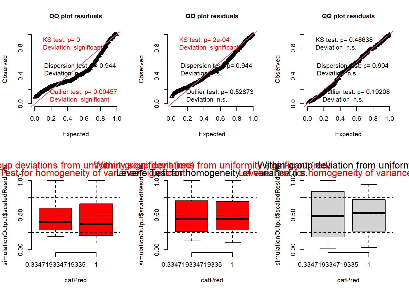

par(mfrow=c(1,1))

It is now very clear that the inverse RT model has a superior fit to the others.

Dataset 3: Custom DHARMa Residuals for GAMLSS

Explanation of Data Context

Though DHARMa is an amazing package and is surprisingly flexible, not every situation is going to have a right-out-of-the-box solution to problems. As it stands, GAMLSS cannot be instantly plugged into the standard functions of DHARMa. Though the gamlss package already contains residual diagnostics plots like worm plots, it would be nice to have residual plots that match our other generalized models. This would be particularly helpful given the robust number of functions in DHARMa that can assess model misfit.

The ingenuity of the DHARMa package is that you can technically create your own custom residuals so long as you have the right ingredients for the job. I show an example below using two fits, with a Gaussian distribution and another alternative with a Box-Cox Cole and Green distribution using a default log link for the conditional mean (BCCGo). This is a more flexible three-parameter distribution for this particular modeling problem, so it may approximate the relationship more flexibly. Though some more robust fits of the response variable are possible (see Chapter 1 of Stasinopoulos et al., 2017), I will show a simpler model that still fits the data quite will compared to a standard Gaussian model.

The model we are trying to fit is one which predicts the rent prices based on the floor an apartment is on. There is probably some psychological factor at play here. Perhaps living on a higher floor means you have to take more steps up the staircase, which will lower the price. Or maybe living on a higher floor means being away from insects like roaches in densely populated bottom floors, which may increase the price for higher floors. Or living on higher floors offers a more scenic view, which results in higher rent prices. We can find out directly by modeling this ourselves. The data used comes from the rent data from the gamlss.data package.

It may help to plot the raw (marginal) distribution first before moving on to modeling.

plot(
  rent$Fl,
  rent$R,
  col = "gray",
  pch = 19,
  xlab = "Floor",
  ylab = "Rent Price",
  main = "Raw Scatterplot of Rent Prices by Floor"
)

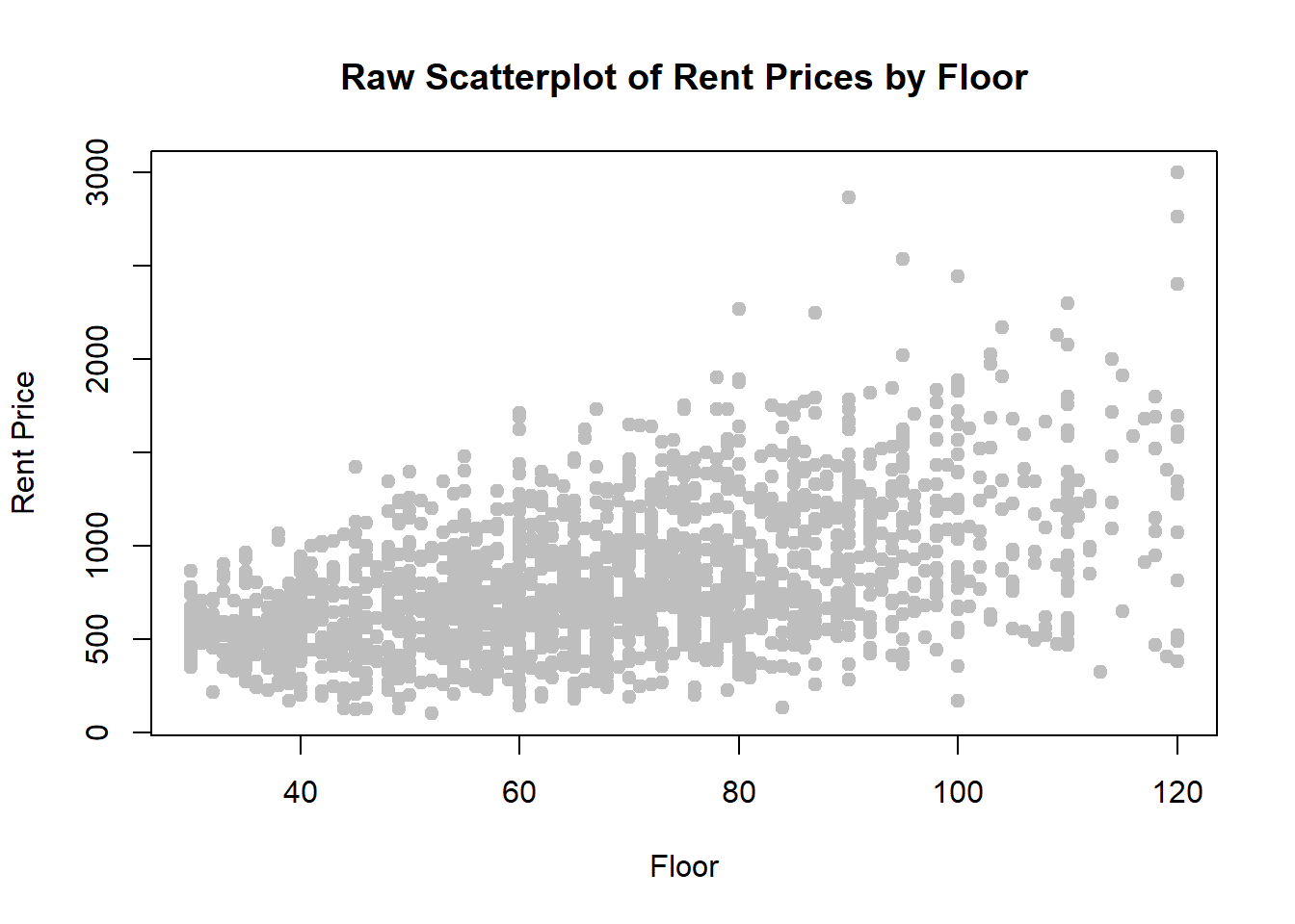
We see that the association between floor and rent prices already looks positive (so living on a higher floor indeed translates to higher rents). The dispersion of the data is a bit unequal at times. We can see for example that there is more data packed into the left of the plot than the right. Because there are so many observations, its unclear what the variance relationship is here, so a more flexible model may be beneficial.

Model 1: Fitting a Gaussian GAMLSS

First, let’s begin with a less ideal model. This GAMLSS will fit the conditional mean and conditional variance of the model using a Gaussian residual family. What this means is that rather than predicting what the average rent should be, we can also predict what the average variation of that rent should be as well.

The first argument specifies the conditional mean (like most models in R) and the second part is a formula for estimating the conditional variance (in this case, we just use the nonlinear effect of floor).

#### Fit GAMLSS Model ####
fit.gamlss.1 <- gamlss(
  R ~ pb(Fl),
  sigma.fo = ~ pb(Fl),
  data = rent
)

GAMLSS-RS iteration 1: Global Deviance = 28153.55 
GAMLSS-RS iteration 2: Global Deviance = 28147.54 
GAMLSS-RS iteration 3: Global Deviance = 28147.38 
GAMLSS-RS iteration 4: Global Deviance = 28147.37 
GAMLSS-RS iteration 5: Global Deviance = 28147.37

We can plot the model’s conditional mean like so, which shows that rental prices increase as the apartment gets higher off the ground:

term.plot(fit.gamlss.1, what = "mu")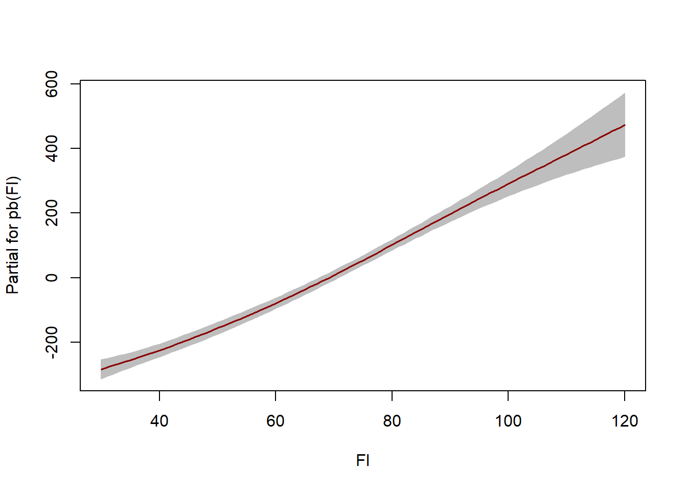

The nice part about GAMLSS is that you can also look at how the variance shifts with the predictor. In this case it is a nonlinear association:

term.plot(fit.gamlss.1, what = "sigma")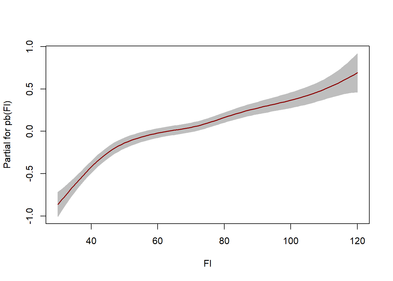

First, let’s extract the parameters from the model directly and save them as objects.

#### Extract Fitted Parameters ####
mu.hat.1 <- fitted(fit.gamlss.1, "mu")
sigma.hat.1 <- fitted(fit.gamlss.1, "sigma")
n.sim.1 <- 250

From here, we can construct something similar to simulate() using the replicate() function. This runs the same function as many times we want (in this case, 250 times). Within replicate(), we estimate a normal distribution with rNO() from the gamlss.dist package. We use the number of observations in the data for the first argument, the estimated conditional mean for the second argument, and the estimated conditional variance for the third argument. This gets saved as sim.matrix.1.

sim.matrix.1 <- replicate(
  n.sim.1, # run this simulation 250 times...
  rNO(
    n = length(mu.hat.1),
    mu = mu.hat.1,
    sigma = sigma.hat.1
    ) # ...using these parameters
)

From here, we just feed the simulations into the createDHARMa() function. We supply the simulations into the first argument, the observed response in the second argument, and the fitted response we want with mu.hat.1.

#### Feed to DHARMa ####
res.1 <- createDHARMa(
  simulatedResponse = sim.matrix.1,
  observedResponse = rent$R,
  fittedPredictedResponse = mu.hat.1
)

All we have to do from here is plot the DHARMa object like we always do.

#### Plot Standard DHARMa Plots ####
plot(res.1)

Warning in newton(lsp = lsp, X = G$X, y = G$y, Eb = G$Eb, UrS = G$UrS, L = G$L,
: Fitting terminated with step failure - check results carefully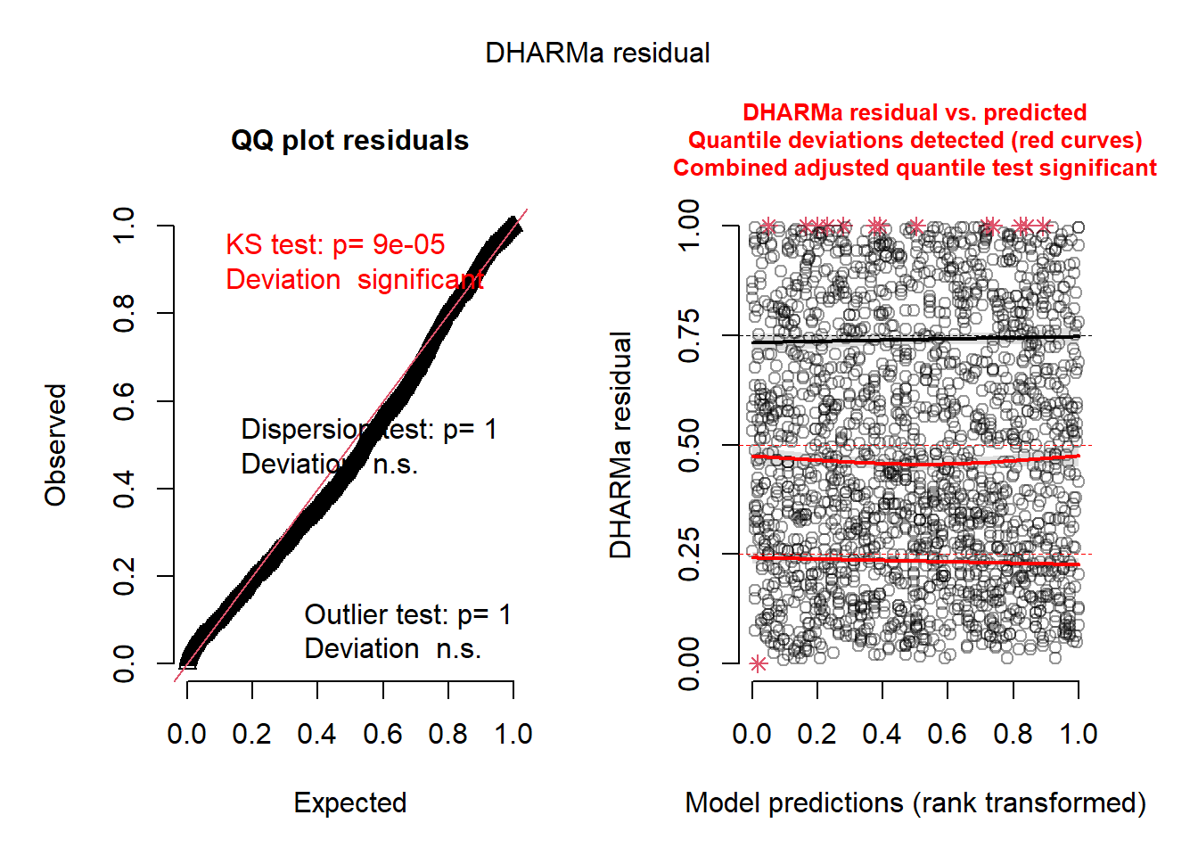

The model isn’t terrible but it certainly isn’t perfect either. We see the most sizeable deviations from expectation in the middle of the distribution near the median. Its possible that fitting with a different distribution would fare better.

Model 2: Using a More Flexible GAMLSS

Lets use a better-fitting model next. We will do almost the exact same thing as before. For this model, we will use the BCCGo family and estimate the variance/skew freely. The only major differences in code are the family = BCCGo argument added to gamlss(), the nu.formula for estimating the other moments of the distribution, and the nu parameter for simulation. This nu paramater allows us to more flexibly model skew/variance. Otherwise the code is the same, which I pack into this single code block.

#### Fit GAMLSS Model ####
fit.gamlss.2 <- gamlss(
  R ~ pb(Fl),
  sigma.fo = ~ pb(Fl),
  nu.formula = ~ pb(Fl), # added this
  data = rent,
  family = BCCGo # and this
)

GAMLSS-RS iteration 1: Global Deviance = 28092.9 
GAMLSS-RS iteration 2: Global Deviance = 28032.47 
GAMLSS-RS iteration 3: Global Deviance = 28030.85 
GAMLSS-RS iteration 4: Global Deviance = 28030.76 
GAMLSS-RS iteration 5: Global Deviance = 28030.75 
GAMLSS-RS iteration 6: Global Deviance = 28030.75

#### Extract Fitted Parameters ####
mu.hat.2 <- fitted(fit.gamlss.2, "mu")
sigma.hat.2 <- fitted(fit.gamlss.2, "sigma")
nu.hat.2 <- fitted(fit.gamlss.2, "sigma") # new parameter from model
n.sim.2 <- 250

#### Simulate Multiple Responses Based on Model ####
sim.matrix.2 <- replicate(
  n.sim.2,
  rBCCGo(
    length(mu.hat.2),
    mu = mu.hat.2,
    sigma = sigma.hat.2,
    nu = nu.hat.2
    ) # simulate BCCGo w/ parameters
  )

#### Feed to DHARMa ####
res.2 <- createDHARMa(
  simulatedResponse = sim.matrix.2,
  observedResponse = rent$R,
  fittedPredictedResponse = mu.hat.2
)

#### Plot Standard DHARMa Plots ####
plot(res.2)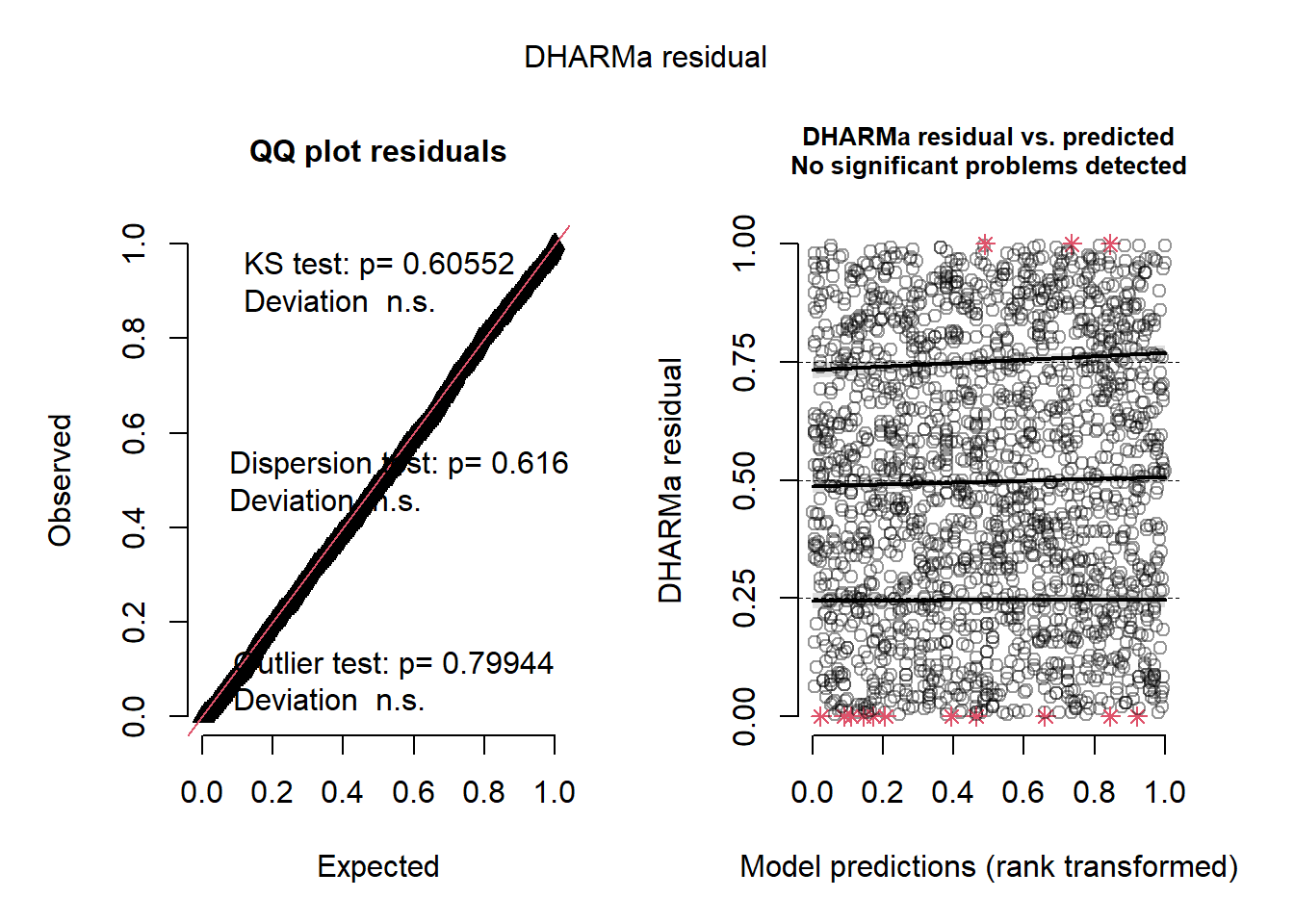

While we do see some outliers in the right plot, this model still fits generally better than the previous one.

Bonus: Fitting a PIG Model for Extreme Skew

Now that we know how to use customized residuals in DHARMa, we can return to our previous count model that had lingering problems of overdispersion. We will once again use the GAMLSS framework for the Nettle data, but this time we will use a Poisson Inverse Gaussian (PIG) model to improve what we had. Like the negative binomial model, the PIG uses a mixture distribution. However, the big difference is that the standard negative binomial model (NB2) model uses a Poisson-Gamma mixture distribution while the PIG uses a Poisson-Inverse Gaussian mixture. The latter is better suited for very right-skewed counts because of the inverse Gaussian part of the model (Hilbe, 2014, p.10-11).

To fit the PIG GAMLSS, we use the following code:

fit.pig <- gamlss(
  formula = Langs ~ MGS + offset(Area),
  data = nettle,
  family = PIG
)

GAMLSS-RS iteration 1: Global Deviance = 765.2821 
GAMLSS-RS iteration 2: Global Deviance = 763.0167 
GAMLSS-RS iteration 3: Global Deviance = 762.2901 
GAMLSS-RS iteration 4: Global Deviance = 762.1469 
GAMLSS-RS iteration 5: Global Deviance = 762.1267 
GAMLSS-RS iteration 6: Global Deviance = 762.1244 
GAMLSS-RS iteration 7: Global Deviance = 762.124

Now we do what we did before with the previous GAMLSS…we simulate the distribution and use replicate() to do the heavy lifting. Note however that because this is a more complicated fit, the process is a lot slower. I set the number of simulations to be 100 to improve speed, but it is recommended to keep the number the same or higher as the default in DHARMa for a final residual analysis.

#### Get Parameters ####
mu.pig <- fitted(fit.pig, "mu")
sigma.pig <- fitted(fit.pig, "sigma")
n.sim.pig <- 100

#### Simulate ####
sim.matrix.pig <- replicate(
  n = n.sim.pig,
  rPIG(
    n = length(mu.pig),
    mu = mu.pig,
    sigma = sigma.pig
    )
  )

#### Feed to DHARMa ####
res.pig <- createDHARMa(
  simulatedResponse = sim.matrix.pig,
  observedResponse = nettle$Langs,
  fittedPredictedResponse = mu.pig
)

#### Plot Standard DHARMa Plots ####
plot(res.pig)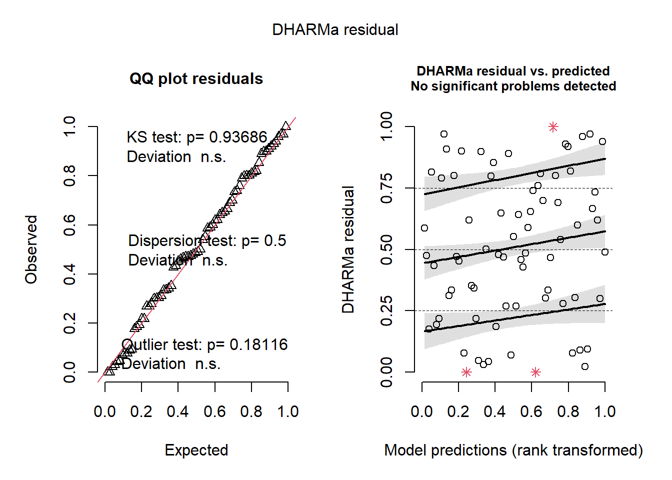

As it stands, this model looks slightly worse. The quantile regression lines all have positive magnitude, but are at least all parallel. There are also some outliers which weren’t present before. We could see if the dispersion has improved enough to consider it as an alternative model.

testDispersion(res.pig)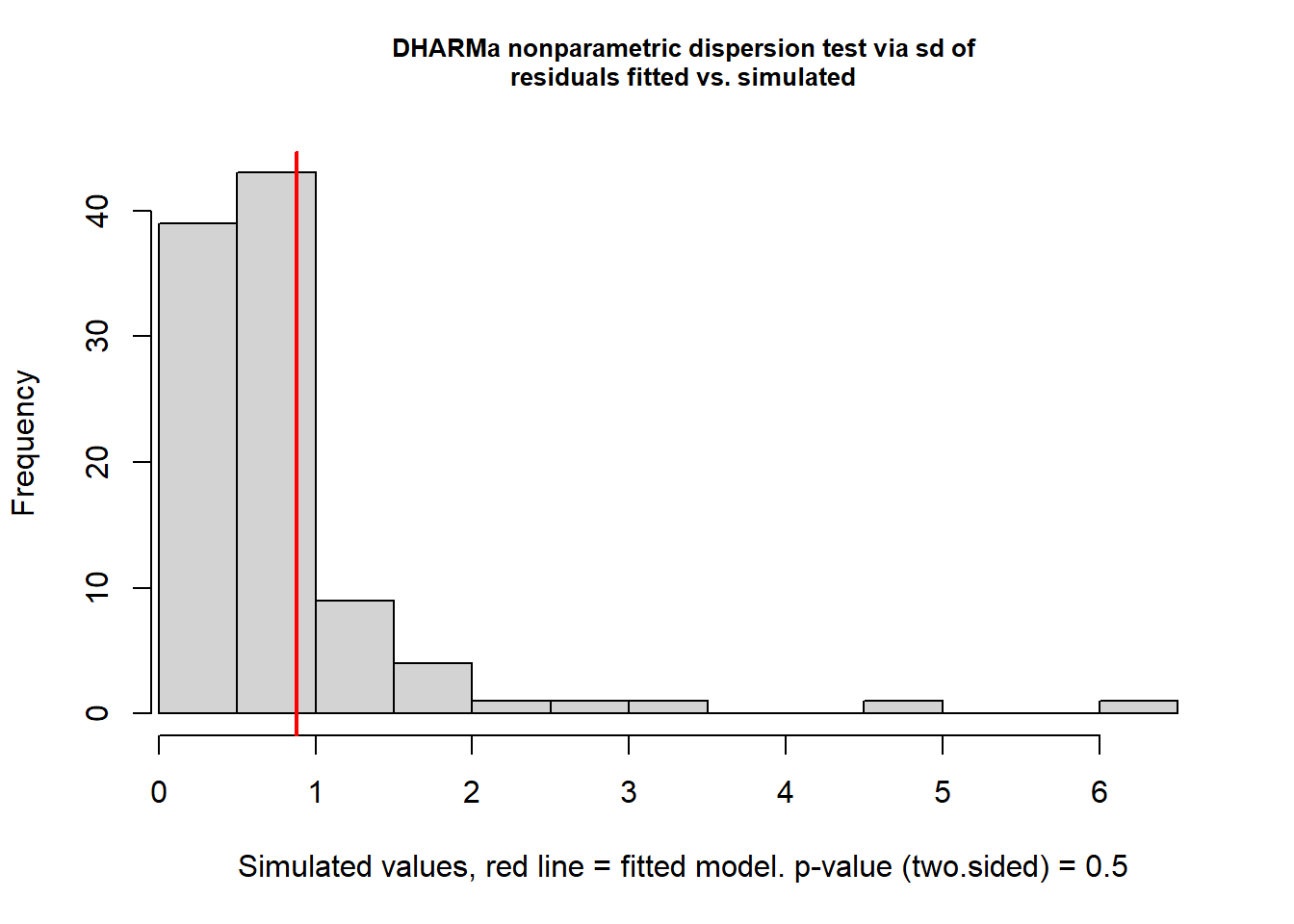


    DHARMa nonparametric dispersion test via sd of residuals fitted vs.
    simulated

data:  simulationOutput
dispersion = 1.078, p-value = 0.5
alternative hypothesis: two.sided

The dispersion for this model is as good as it gets. Note that in some simulations the model was underdispersed, which means this model may have been corrected too much by the PIG fit. We could also check the AIC/BIC of the two models to see if one is vastly superior to the others. If the difference is not huge, its probably better to stick with the negative binomial model since it already offers a huge advantage compared to other others (Hilbe, 2014, p.40).

AIC(fit.nb, fit.pig)

        df      AIC
fit.nb   3 771.8767
fit.pig  3 768.1240

BIC(fit.nb, fit.pig)

        df      BIC
fit.nb   3 778.7889
fit.pig  3 775.0362

Given the tiny differences in AIC/BIC, the potential increase in model misfit, and the complexity of the PIG model, it appears safer to simply retain the more parsimonious negative binomial model. There are likely other fits which could improve the model further, but this is probably as ideal as we can get the fit.

References

Baayen, R.H., Davidson, D.J., & Bates, D.M. (2008). Mixed-effects modeling with crossed random effects for subjects and items. Journal of memory and language, 59(4), 390-412.

Baayen, H.R., & Milin, P. (2010). Analyzing reaction times. International Journal of Psychological Research, 3(2), 12–28. https://doi.org/10.21500/20112084.807

Gelman, A., Hill, J., & Vehtari, A. (2022). Regression and other stories. Cambridge University Press.

Greenwald, A.G., & Banaji, M.R. (1995). Implicit social cognition: Attitudes, self-esteem, and stereotypes. Psychological Review, 102, 4-27. https://doi.org/10.1037/0033-295X.102.1.4

Greenwald, A.G., McGhee, D.E., & Schwartz, J.K.L. (1998). Measuring individual differences in implicit cognition: The Implicit Association Test. Journal of Personality and Social Psychology, 74, 1464-1480. https://doi.org/10.1037//0022-3514.74.6.1464

Hilbe, J. M. (2014). Modeling count data. Cambridge Univ. Press.

Mair P. (2020). MPsychoR: Modern Psychometrics with R. https://doi.org/10.32614/CRAN.package.MPsychoR, R package version 0.10-8, https://CRAN.R-project.org/package=MPsychoR.

Nettle, D. (1999). Linguistic diversity. Oxford University Press.

Nosek, B.A., Banaji, M.R., & Greenwald, A.G. (2002). Harvesting implicit group attitudes and beliefs from a demonstration web site. Group Dynamics: Theory, Research, and Practice, 6, 101-115.

Stasinopoulos, M.D., Rigby, R.A., Heller, G.Z., Voudouris, V., & Bastiani, F.D. (2017). Flexible regression and smoothing: Using GAMLSS in R. CRC Press.

Winter, B. (2019). Statistics for linguists: An introduction using R (1st ed.). Routledge.