install.packages("DHARMa")
library(DHARMa)Getting Started
Introduction
This page details the most basic functions of the DHARMa package (Hartig, 2017). It is recommended to start here before moving on to other pages. As the demonstrations here focus on an ideal scenario with a basic dataset, it is recommended after to navigate to the Simulated Data and Real Data pages for more robust examples.
Foundational Functions of DHARMa
Setting Up DHARMa
First, you will need to install and load the DHARMa package in R with the following code.
Ensure that you have the latest version of R, RStudio, and the DHARMa package before running any analyses.
Getting the Residuals
From here, we fit a basic regression model (more realistic examples are shown in the Simulated Data and Real Data sections). We will use the attitude data that already comes with R (Chatterjee & Price, 1977). We will try to predict how a finance company is rated based on the number of raises, complaints, privileges, and advances that are reported by employees.
This will be fit with the glm() function in R with a Poisson regression. These models are primarily used to predict count variables such as our response (Westfall & Arias, 2020). The first argument specifies the regression formula, the second specifies the data used, and the third specifies the distribution to be used (here the Poisson).
fit <- glm(
  formula = rating ~ raises + complaints + privileges + advance,
  data = attitude,
  family = poisson()
)
From here, we just get the residuals by plugging our fit object into simulateResiduals(). We will save this object as sim to use later.
sim <- simulateResiduals(fit)Standard DHARMa Plots
From here, we will produce two of the most common plots used in DHARMa by using plot() on our sim object.
plot(sim)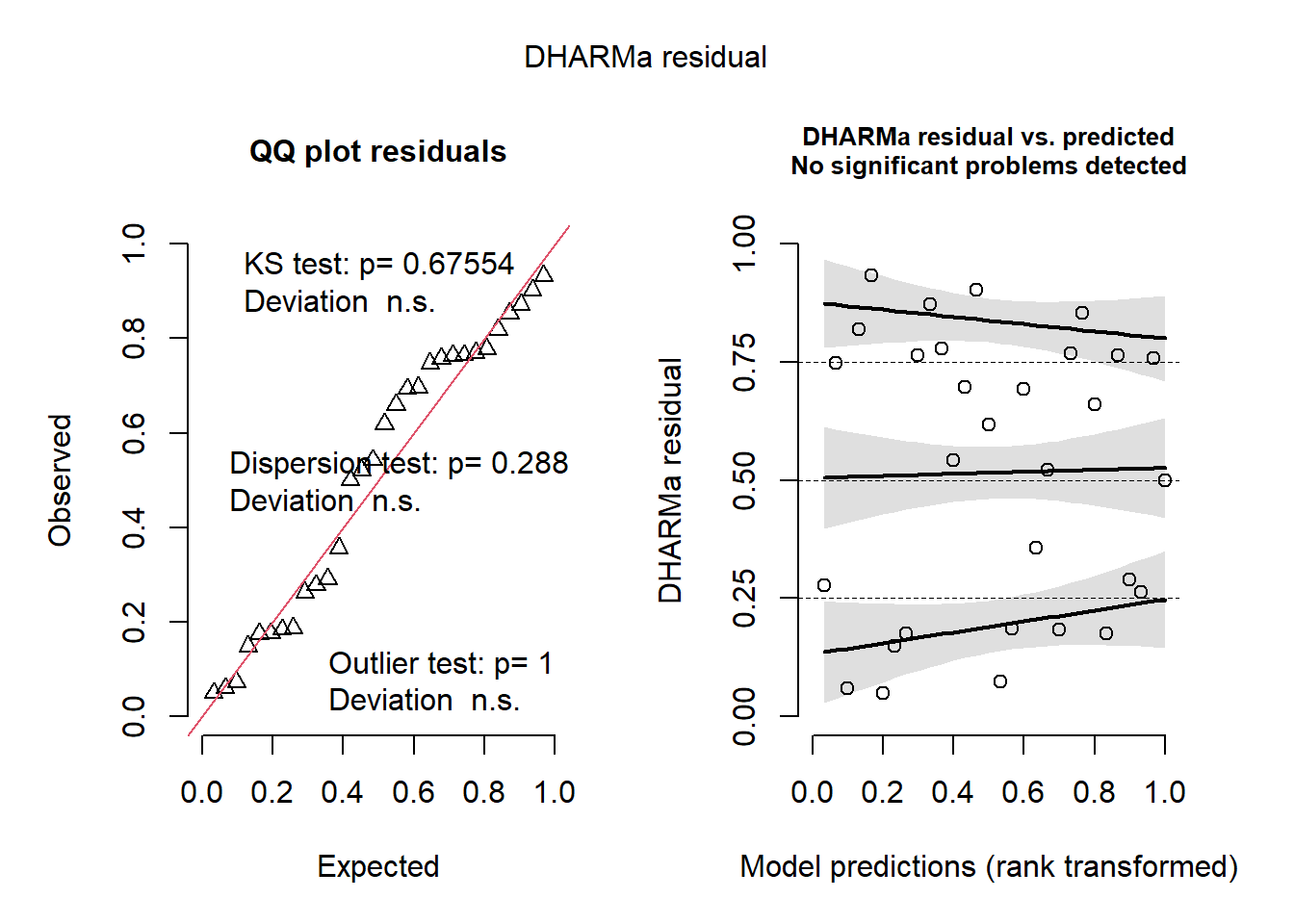
The first plot is a QQ plot and shares a very similar interpretation as standard QQ plots (using a uniform distribution instead of a normal distribution). If the dots do not appreciably deviate from the red line, then the residuals correctly approximate a uniform distribution and we at least have some assurance our model is fit fine. This is similar to checking the normality assumption in ordinary least squares (OLS) regression (see Chapter 4 of Westfall & Arias, 2020).
The right plot is very similar to a fitted vs residuals plot in OLS regression (see Chapter 4 of Westfall & Arias, 2020). However, this plot by default comes with a QGAM (Fasiolo et al., 2021) to observe if there are patterns across the distribution of residuals. We usually want the solid black lines to be horizontal and parallel to each other. If they are curvy or differ in magnitude/direction, then this can be problematic. In this case, both plots seem to have no major issues. If there are differences in magnitude or curves in the lines, this can be attributed to nonlinearity or heteroscedascity. If red stars are visible, these are indicators of outliers (Hartig, 2017).
You can also plot these individually for closer visual inspection. The left plot can be produced with the below code. Each comes with statistical tests to assess fit, though it is advised to be cautious with these tests. They are sensitive to sample size and are best not used as a default for assumption checks (Hartig, 2017; Shatz, 2024).
testUniformity(sim)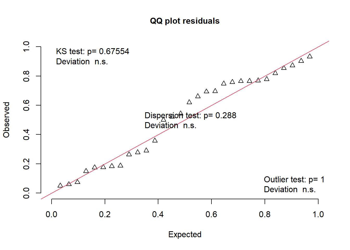
    Exact one-sample Kolmogorov-Smirnov test

data:  simulationOutput$scaledResiduals
D = 0.12661, p-value = 0.6755
alternative hypothesis: two-sided
The right plot can be produced with this function:
testQuantiles(sim)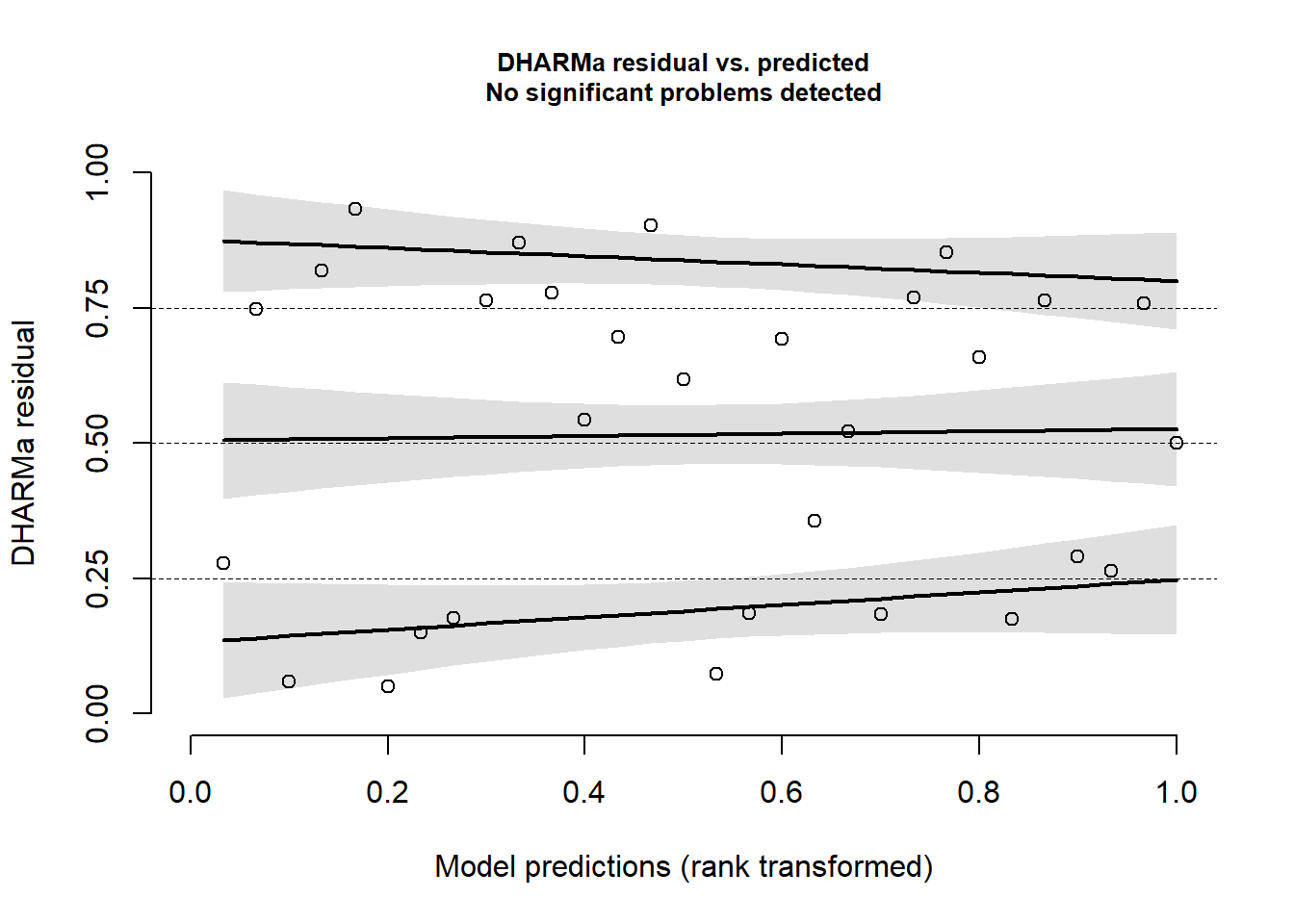
    Test for location of quantiles via qgam

data:  res
p-value = 0.3592
alternative hypothesis: both
These plots can get murky if there are many terms in the model such as the one we fit. To inspect the residuals conditional upon a specific predictor, we can use the plotResiduals() function and use the form argument to tell R which predictor to consider. Here we check the complaints predictor specifically, which shows no obvious issues.
plotResiduals(sim, form = attitude$complaints)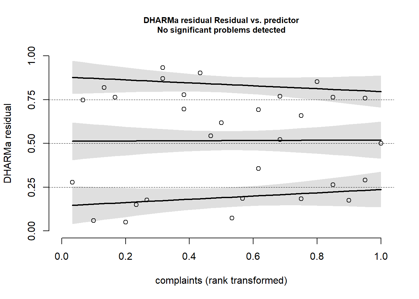
You probably noticed that the first plot included multiple tests, including for dispersion, normality, and outliers. We provide more details about these checks below.
Going Further: Helpful Functions in DHARMa
Checking Dispersion
Dispersion checks are used to assess if a model is underfitting (the model is too basic) or overfitting (the model is too complex). Our above model uses a Poisson regression, and this requires satisfying certain assumptions such as equidispersion. For the Poisson distribution, this means that the mean and the variance \(\lambda\) are assumed to be approximately equal. To assess if this is true, we simply check that the dispersion is equal to 1 and visualize this with plots. This can be straightforwardly visualized and tested with the testDispersion() function in DHARMa.
testDispersion(sim)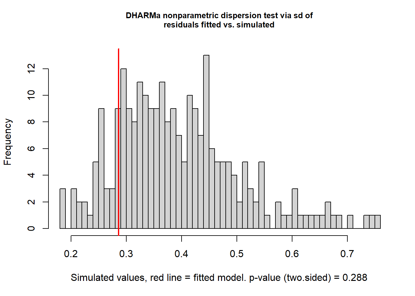
    DHARMa nonparametric dispersion test via sd of residuals fitted vs.
    simulated

data:  simulationOutput
dispersion = 0.72676, p-value = 0.288
alternative hypothesis: two.sided
We usually want a dispersion value that is relatively close to 1, which suggests that the mean is close to equal to the variance (Khan et al., 2026). More specifically, DHARMa checks to see if the simulated dispersion (from the randomized quantile residuals) matches that of the observed data. Our output suggests that the model is likely safe. The red line indicates the degree of over- or underdispersion. If the red line deviates substantially to the right of the histogram, then the model is more overdispersed. If the red line deviates substantially to the left, then the model is underdispersed. In this case, the red line is situated near the center of the distribution and is likely safe. Examples of extreme cases are highlighted on the DHARMa vignette page (Hartig, 2017).
As noted earlier, this can generally occur in models as a consequence of mis-specification or overfitting (Hartig, 2017). Therefore, it may be beneficial to assess other problems with model fit if this comes from models that don’t model count responses.
Checking Outliers
The DHARMa package also checks for outliers. This can be assessed quickly with the testOutliers() function, which marks outliers in the given histogram in red.
testOutliers(sim)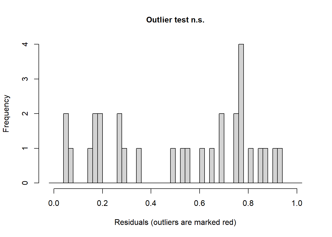
    DHARMa bootstrapped outlier test

data:  sim
outliers at both margin(s) = 0, observations = 30, p-value = 1
alternative hypothesis: two.sided
 percent confidence interval:
 0.00000000 0.05083333
sample estimates:
outlier frequency (expected: 0.0106666666666667 )
                                                0
Since the randomized quantile residuals are normally only supposed to have values between 0 and 1 (see “What is DHARMa?” page for details), residuals that reach these values are considered outliers. Take caution: DHARMa does not know how outlying these points are due to the boundedness of the residual (see documentation for this function). Therefore, further checks, particularly with visualization or Cook’s distance, can help determine if these outliers are indeed impactful on the model. Cook’s distance is one generalizable measure that can be directly calculated on the fitted model without DHARMa, such as below.
plot(
  cooks.distance(fit),
  type = "h",
  main = "Cook's Distance",
  ylab = "Distance"
  )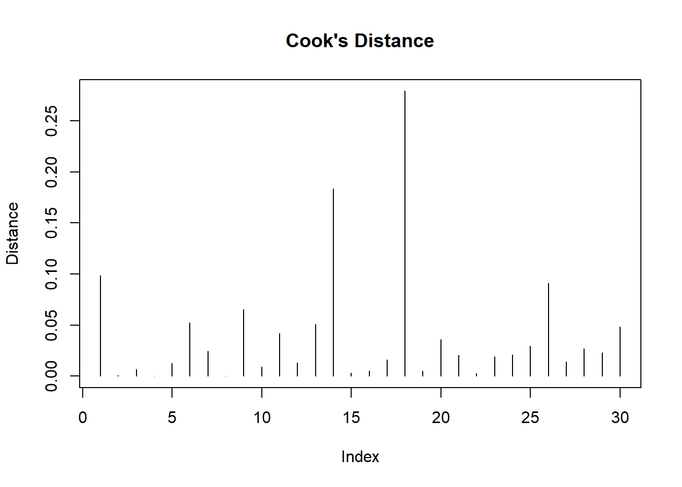
Values above .5 can be considered influential and above 1 may be substantially so. Here we do not have any issues.
Check Autocorrelation
There are three primary autocorrelation checks in DHARMa:
testTemporalAutocorrelation(): Used to assess the statistical relationship of a variable with itself over time.testSpatialAutocorrelation(): Used to assess the statistical relationship of a variable with itself over space.testPhylogeneticAutocorrelation(): Used to assess the statistical relationship of a variable with itself among species.
Psychology research typically deals most with temporal autocorrelation, such as correlated observations across experimental trials (Baayen et al., 2017). We shouldn’t expect this to be an issue for our above model. However, let’s imagine the employees were surveyed across 30 days. We can add this into the original dataset and refit the model.
#### Create New Data with "Day" Variable ####
attitudes.2 <- attitude
attitudes.2$time <- 1:30

#### Refit Model ####
fit.2 <- glm(
  formula = rating ~ raises + complaints + privileges + advance,
  data = attitudes.2,
  family = poisson()
)
Then we just plot the model into the first part of the testTemporalAutocorrelation() function, followed by the time variable in our data.
testTemporalAutocorrelation(sim, time = attitudes.2$time)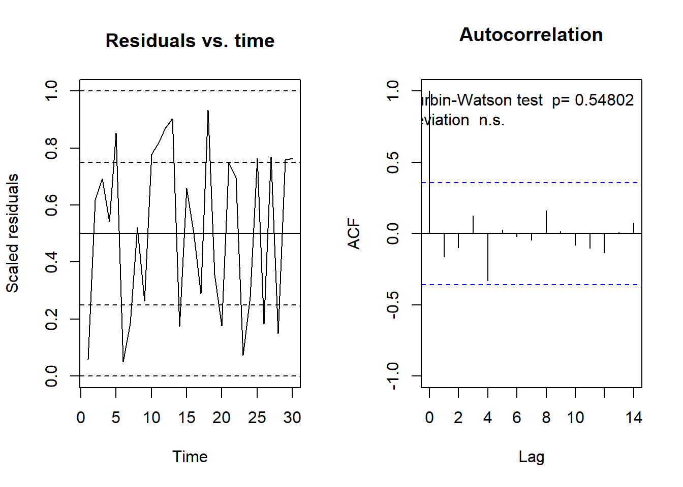
    Durbin-Watson test

data:  simulationOutput$scaledResiduals ~ 1
DW = 2.2165, p-value = 0.548
alternative hypothesis: true autocorrelation is not 0
The left visualization plots the time (day) against the residuals. The right visualization plots the the degree of correlation with observations and their past values. For example, the first lag (lag = 0) has a correlation of 1 because any observation will be perfectly correlated with itself. When lag = 1, this is an observation shifted by one time step (here one day). There should be no relationship between an observation and its associated increases in this lag unless unmodeled temporal trends (e.g. time series) are present. As to be expected, we see no obvious issues of autocorrelation in either plot. Serious issues arise when we observe a pattern in the left plot or non-random, large bars that exceed the dashed blue line in the right plot.
Summary
On this page, we looked at some of the core functions of DHARMa. These functions will serve most of a researcher’s purposes when engaging in model criticism. To observe how these functions are used in practice, please see the Simulated Data and Real Data sections of the website.
References
Baayen, H., Vasishth, S., Kliegl, R., & Bates, D. (2017). The cave of shadows: Addressing the human factor with generalized additive mixed models. Journal of Memory and Language, 94, 206–234. https://doi.org/10.1016/j.jml.2016.11.006
Chatterjee, S. and Price, B. (1977) Regression Analysis by Example. New York: Wiley.
Fasiolo, M., Wood, S.N., Zaffran, M., Nedellec, R., & Goude, Y. (2021). Qgam: Bayesian nonparametric quantile regression modeling in R. Journal of Statistical Software, 100(9). https://doi.org/10.18637/jss.v100.i09
Hartig, F. (2017). DHARMa: Residual diagnostics for hierarchical (multi-level/mixed) regression models. https://cran.r-project.org/web/packages/DHARMa/vignettes/DHARMa.html
Khan, N.M., Baldi, I., Chiaruttini, M.V., & Gregori, D. (2026). Residuals and overdispersion in generalized linear models. In N.M. Khan, I. Baldi, M.V. Chiaruttini, & D. Gregori, Classical and Bayesian Statistical Approaches in Infectious Disease Data Analysis (pp. 169–190). Springer Nature Switzerland. https://doi.org/10.1007/978-3-032-06747-0_6
Shatz, I. (2024). Assumption-checking rather than (just) testing: The importance of visualization and effect size in statistical diagnostics. Behavior Research Methods, 56(2), 826–845. https://doi.org/10.3758/s13428-023-02072-x